Introduction
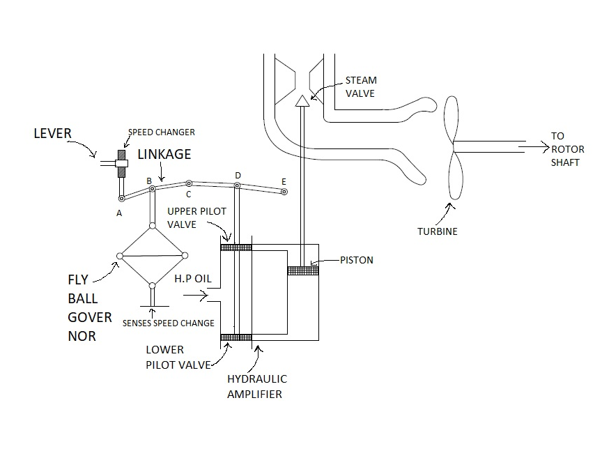
The generator turbine governor control regulates rotational speed in response to changing load conditions. The governor output signal manipulates the position of a steam inlet valve or nozzles which in turn regulates the steam flow to the turbine.
Turbine-generator units operating in a power system contain stored kinetic energy due to their rotating masses. If the system load suddenly increases, stored kinetic energy is released to initially supply the load increase. Also, the electrical torque Te of each turbine-generating unit increases to supply the load increase, while the mechanical torque Tm of the turbine initially remains constant.
Generator Dynamics
From Newton’s second law, Jα = Tm – Te, the acceleration α is therefore negative. That is, each turbine-generator decelerates and the rotor speed drops as kinetic energy is released to supply the load increase. The electrical frequency of each generator, which is proportional to rotor speed for synchronous machines, also drops.
From this, we conclude that either rotor speed or generator frequency indicates a balance or imbalance of generator electrical torque Te and turbine mechanical torque Tm.
If speed or frequency is decreasing, then Te is greater than Tm (neglecting generator losses). Similarly, if speed or frequency is increasing, Te is less than Tm. Accordingly, generator frequency is an appropriate control signal for governing the mechanical output power of the turbine.
The steady-state frequency-power relation for turbine-governor control is:
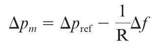
where ∆f is the change in frequency, ∆Pm is the change in turbine mechanical power output, and ∆Pref is the change in a reference power setting. ‘R’ is called the regulation constant.
Below figure shows the family of curves for above equation, with ∆Pref as a parameter. Note that when ∆Pref is fixed, ∆Pm is directly proportional to the drop in frequency.
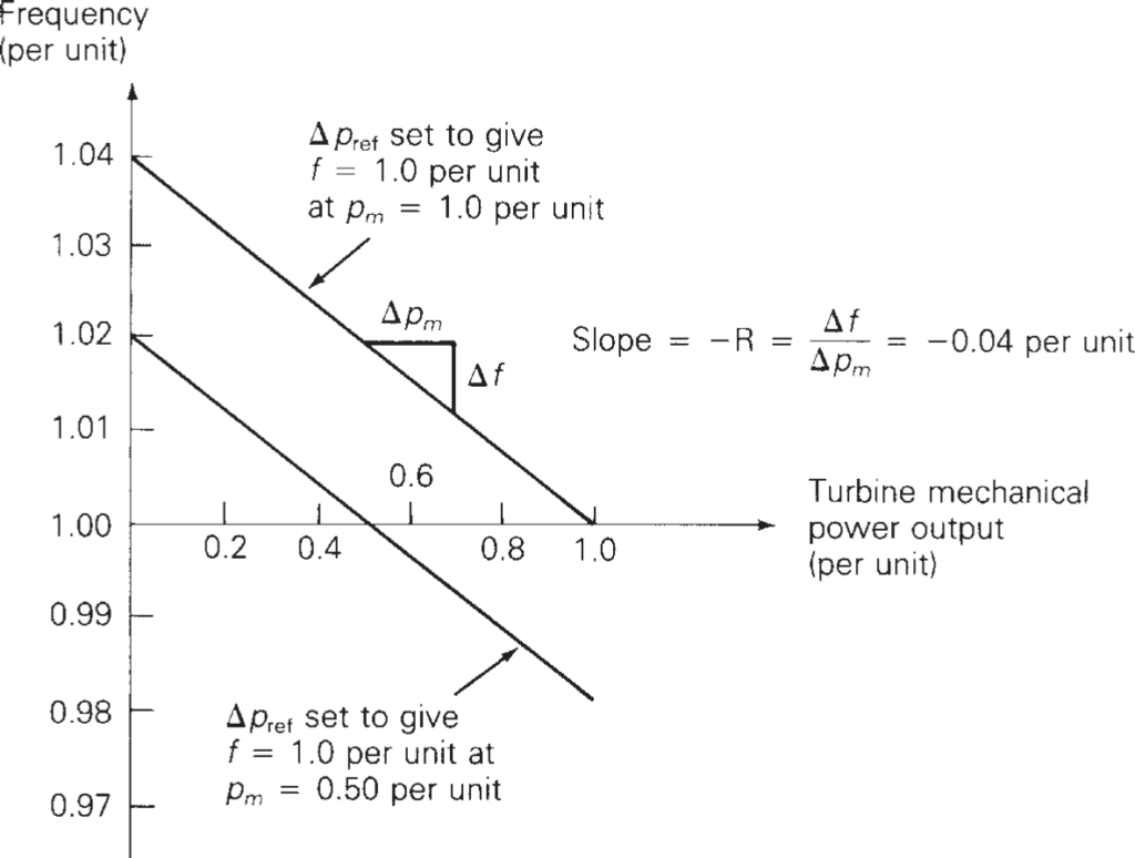
Above figure illustrates a steady-state frequency-power relation. When an electrical load change occurs, the turbine-generator rotor accelerates or decelerates, and frequency undergoes a transient disturbance. Under normal operating conditions, the rotor acceleration eventually becomes zero, and the frequency reaches a new steady-state, shown in the figure.
The regulation constant ‘R’ is the negative of the slope of the ∆f versus ∆Pm curves as per above figure. The units of R are Hz/MW when ∆f is in Hz and ∆Pm is in MW. When ∆f and ∆Pm are given in per-unit, however, R is also in per-unit.
Frequency-Power Relation of an Interconnected Power System
The steady-state frequency-power relation for one area of an interconnected power system can be determined by summing Equation – (1) for each turbine-generating unit in the area. Noting that ∆f is the same for each unit,
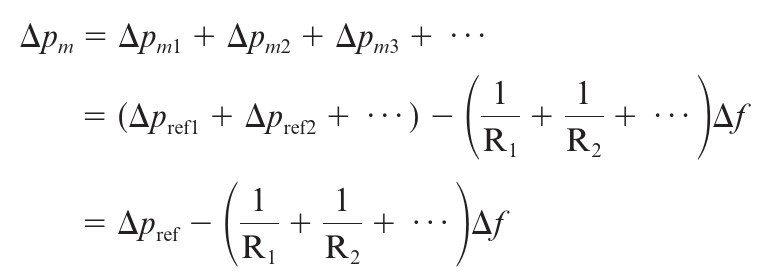
where ∆Pm is the total change in turbine mechanical powers and ∆Pref is the total change in reference power settings within the area. We define the area frequency response characteristic β as:
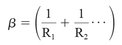
Using Equation – (3) in Equation – (2),
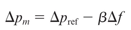
Equation – (4) is the area steady-state frequency-power relation. The units of β are MW/Hz when ∆f is in Hz and ∆Pm is in MW. β can also be given in per-unit.
Turbine Governor Block Diagram
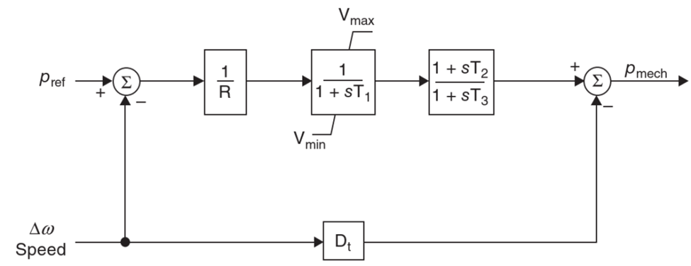
A standard value for the regulation constant is R = 0.05 per unit. When all turbine-generating units have the same per-unit value of R based on their own ratings, then each unit shares total power changes in proportion to its own rating.
Above figure shows a block diagram for a simple steam turbine governor commonly known as the TGOV1 model. The 1/(1 + sT1) models the time delays associated with the governor, where ‘s’ is again the Laplace operator and T1 is the time constant. The limits on the output of this block account for the fact that turbines have minimum and maximum outputs.
The second block diagram models the delays associated with the turbine; for non-reheat turbines T2 should be zero. Typical values are R = 0.05 p.u., T1 = 0.5 seconds, T3 = 0.5 for a non-reheat turbine or T2 = 2.5 and T3 = 7.5 seconds otherwise. Dt, is a turbine damping coefficient that is usually 0.02 or less (often zero).
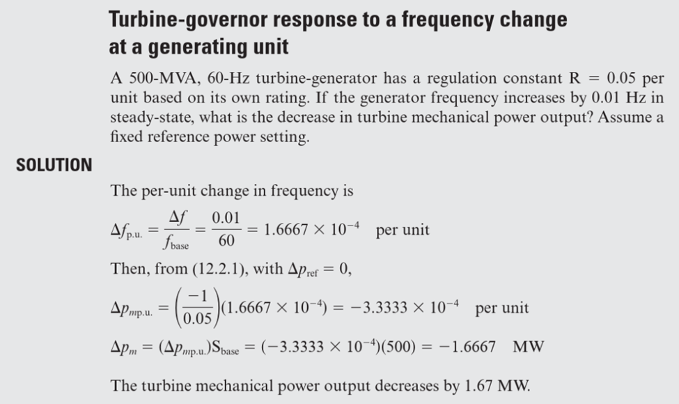
Example